Paper Notes: Proximal Policy Optimization
Notes on PPO
TL;DR
- alternates between sampling data through interaction and optimizing a surrogate objective
- these optimizations are done using mini-batch gradient ascent updates compared to single sample updates in REINFORCE
- doing multiple updates with same trajectory results in large policy updates which are destructive
- proposes a new objective function to enable these mini-batch updates
- implements a clipped surrogate objective which is simpler to implement than TRPO
Background:
Loss function in vanilla policy gradient approach takes following form:
Add policy gradient derivation
The policy $\pi_{\theta}$ is improved by single step gradient ascent updates on the loss $L^{PG}(\theta)$. Performing multiple steps on the loss leads to large policy updates which are destructive.
In TRPO, we create a surrogate objective with a constraint on the size of policy update.
This constraint theoretically can be added as a penalty term and changed to unconstrained optimization problem.
understand why KL divergence is calculated in that order, why not the other way? Since $KL[P,Q] \neq KL[Q,P]$
But it is hard to find a single value of $\beta$ which works well across different problems (or over course of learning for one problem).
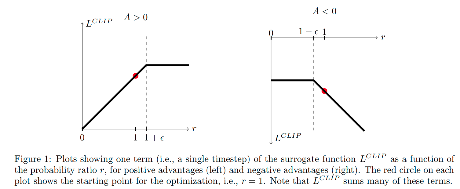
Clipped Surrogate Objective:
Let us call this Conservative Policy Iteration approach as follows:
But without a constraint $L^{CPI}$ will result in large destructive policies if the ratio $r_t(\theta)$ becomes very large. We need to penalize changes which move $r_t(\theta)$ away from 1.
-
First term is same as $L^{CPI}$
- Second term is a clipped ratio $r_t(\theta)$ in between $(1-\epsilon, 1+\epsilon)$ so that ratio is always close to 1. $\epsilon$ is taken to be 0.2 in the paper.
- $\min$ is taken to get a lower bound
Algorithm Details
PPO-clipped objective with parallel actors and synchronized policy updates.
Network Structure:
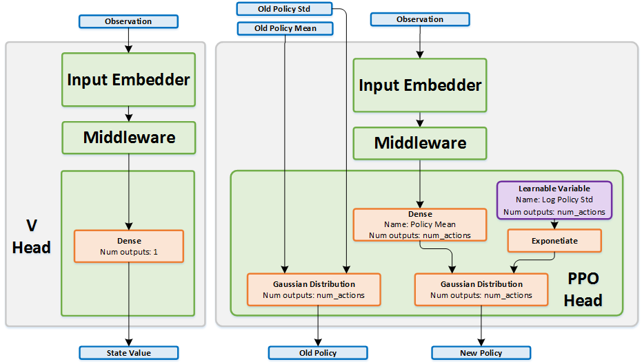
Policy Network:
- input: current state
- output: mean of a gaussian distribution
- architecture:
- Fully connected MLP
- 2 hidden layers with 64 units
tanhnon-linearity- state independent variable for log stddev (take exponential for getting stddev, this is done to keep the stddev from not becoming too large)
Value Network:
- input: current state
- output: value function estimate of the state
- architecture:
- Fully connected MLP
- 2 hidden layers with 64 units
tanhnon-linearity
Note: Policy and Value networks don’t share parameters as mentioned in the original paper.
Initialize policy parameter $\theta$ and value function parameter $\phi$
for $k$ number of epochs:
for parallel actors:
Run policy $\pi_{\theta}$ in environment for $T$ timesteps and collect trajectory $D$
Compute advantage estimates $\hat{A}t$ based on reward-to-go $\hat{R_t}$ and value function $V{\phi}$
Update policy parameter using gradient ascent:
Update value function parameter using gradient descent: