Paper Notes: Attention Is All You Need

NOTE: In-progress

The key idea proposed in the paper is to remove RNN from seq-to-seq task and depend solely on attention mechanism to learn global dependencies between input and output.

This results in the transformer architecture with multiple attention blocks in encoder and decoder.

The fundamental building block for this architecture is the multi-head attention. In order to understand multi-head attention let us first have a look at the scaled dot-product attention.

Scaled Dot-Product Attention:

Attention is described as mapping a query and a set of key - value pairs to an output.

$Attention(Q,K,V) = softmax(\frac{QK^T}{\sqrt{d_k}})V$

where,

​ $Q$: query

​ $K$: key

​ $V$: value

​ $d_k$: dimension of key and query vectors

Let’s break down each term to understand what attention is trying to achieve.

Query and Key Dot-Product:

The first term $QK^T$ is a dot-product between the query and key. The dot-product tells us how close two vectors are in the geometric space - higher the value, closer they are. Intuitively you would want the queries which match with the right key to be close together

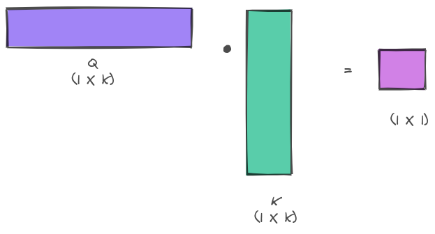
NOTE: assume that $k$ in the image is same as $d_k$

Think about attention as a memory where the data you want to retrieve is stored in terms of values. These values are indexed (think about DB indexes) using its corresponding key. When you want to retrieve the value, you have a query that you are trying to run on the data. So, you take a query and you try to match it with the correct key. If the query and key vectors are close then their dot product should be higher - this is what we want our model to learn.

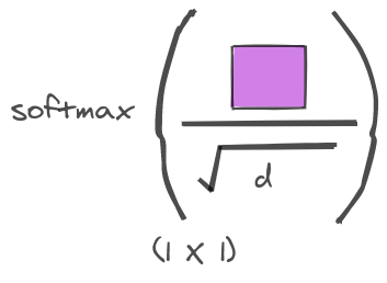
Scaling Factor and Softmax:

Now sometimes when you do dot-product of vectors which are larger in size, you will end up getting extremely high values. The variance of dot product of two vectors of size $d_k$ with 0 mean and 1 variance is $d_k$. So, as the size of vectors increase - the values will become higher. As the values become higher it will push the softmax to regions with smaller gradients. Therefore we need to scale the values using $\sqrt{d_k}$ .

This is passed through softmax function to increase the higher values and keep it in a range of 0 to 1.

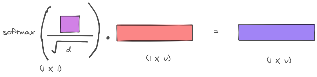
Dot-product with Value:

The final term is multiplied with the Value vector to give us the output vector. Think about this operation as the final look-up the database.

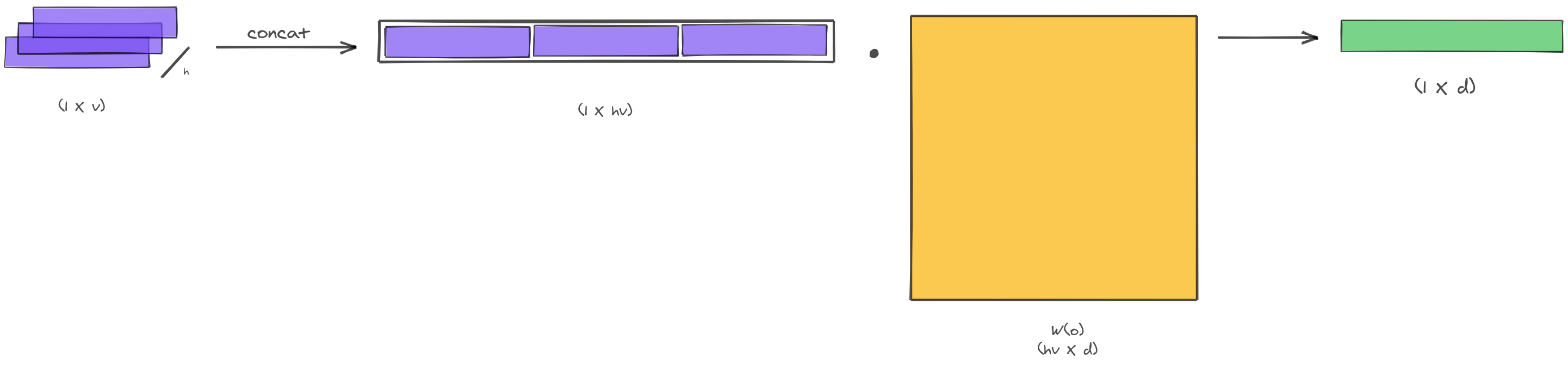
Multi-Head Self Attention:

The first part of multi-head attention is same as the scaled dot-product attention with one modification. Instead of doing the scaled dot-product attention only once, this operation is repeated a number of times (think about different channels) and the final output is concatenated.

In order to facilitate this we take the query, key and value vectors and linearly projected them across different channels.

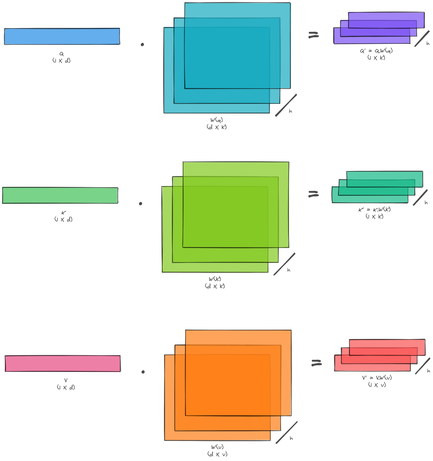
Then we perform the scaled dot-product attention over these projections.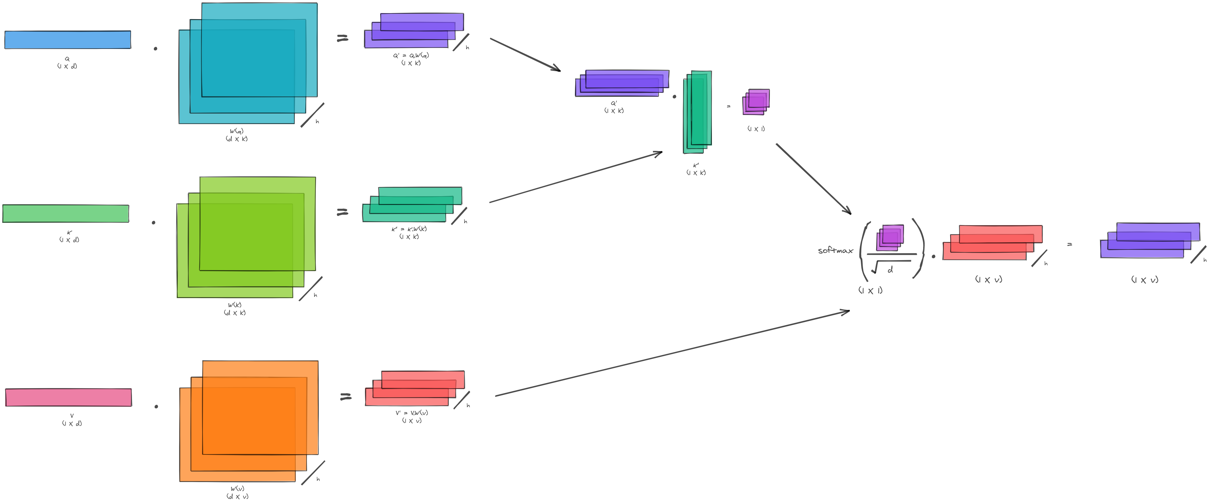

The output from this step is concatenated across these channels and then again linearly projected into the output (to get the desired shape of output vector).

Transformer Architecture

Now that we understand how attention mechanism works, let’s see how it is applied in the transformer network architecture.

Positional Encoding:

The paper proposes to add positional encoding in order to give some information about relative position of the tokens in sequence.

In order to do so we encode each position of the token with a different sinusoidal function. Imagine there are 4 different $d$ dimensional tokens, so we create 4 positional encoding vectors with same dimension $d$. The values of these vectors are given as follows:

For every even dimension of the vector, encode with a sin function

$PE[::2] = \sin{\frac{pos}{10000^{range(0,d,2) / d}}}$

For every odd dimension of the vector, encode with a cos function

$PE[::2] = \cos{\frac{pos}{10000^{range(0,d,2) / d}}}$

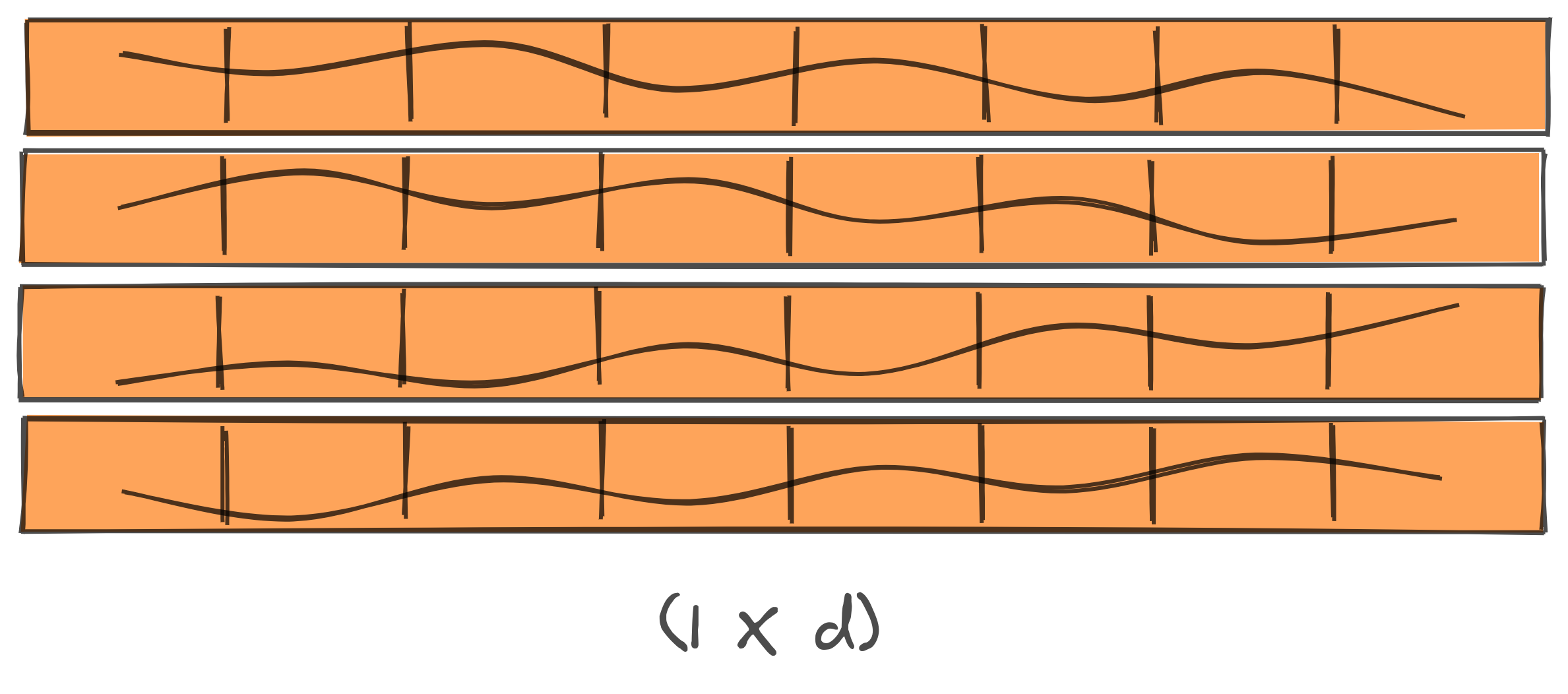
When you add these positional encoding vectors to the input, each input is then linearly translated by this sinusoidal function which is unique for each position. This helps the model to preserve information about relative position of each token. The encodings are applied right after input and output embeddings in both encoder and decoder.

Position-wise Feed-Forward Network:

In both the encoder and decoder, they also have a fully-connected network with relu activation right after the multi-head attention. These transformation use the same parameter for all the positions but they differ for different layers.

$z_1 = xW_1+b_1\\ a_1 = \max(0, z_1)\\ z_2 = a_1 W_2 + b_2$

Encoder:

The encoder module contains 6 identical layers. Each layer has a Multi-Head Attention and Position-wise fully connected network. The sub-layers have residual connections and batch normalization layer on top of that.